Histogram
This notebook shows a few typical uses of mp.histogram with the sample dataset included in the examples folder.
Imports
import matplotlib.pyplot as plt

import mespy as mp


df = mp.load_csv("data/test_misure.csv")
lunghezza = df["lunghezza_mm"]
sigma = df["sigma_mm"]
Basic histogram usage
The only essential argument is the numeric sample used to build the histogram. All other parameters are used to control the plot style, annotations, and layout.
fig, ax = mp.histogram(lunghezza)

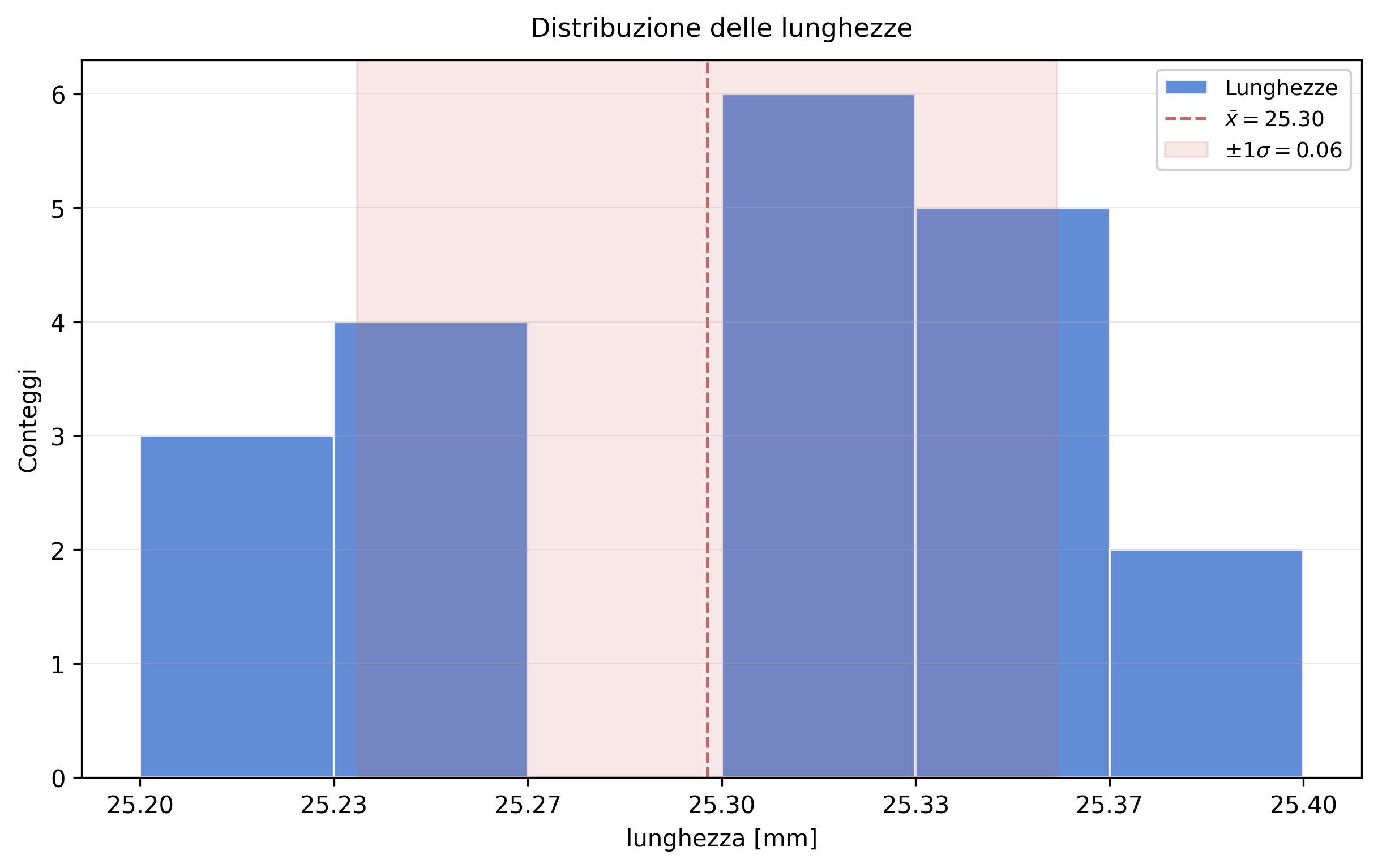
Custom labels and legend
You can change the data label, x axis, title, title size, and legend numeric precision without modifying the rest of the call.
mp.histogram(
    lunghezza,
    label="Lunghezze",
    xlabel="lunghezza [mm]",
    title="Distribuzione delle lunghezze",
    title_fontsize=11,
    decimals=2,
)
(<Figure size 2400x1500 with 1 Axes>,
 <Axes: title={'center': 'Distribuzione delle lunghezze'}, xlabel='lunghezza [mm]', ylabel='Conteggi'>)
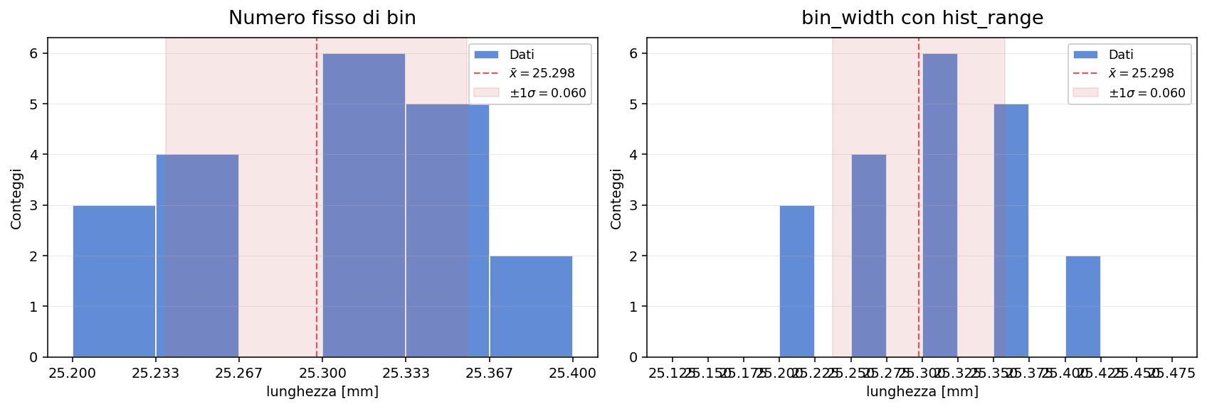
Custom bin settings
bins and bin_width are alternatives: use the former to set the number or strategy of bins directly, and the latter to impose a constant width. hist_range restricts the range used to build the histogram.
fig, (ax_left, ax_right) = plt.subplots(
    1,
    2,
    figsize=(12, 4),
    dpi=140,
    constrained_layout=True,
)

mp.histogram(
    lunghezza,
    bins=6,
    xlabel="lunghezza [mm]",
    title="Numero fisso di bin",
    ax=ax_left,
)

mp.histogram(
    lunghezza,
    bin_width=0.025,
    hist_range=(25.15, 25.45),
    xlabel="lunghezza [mm]",
    title="bin_width con hist_range",
    ax=ax_right,
)

fig
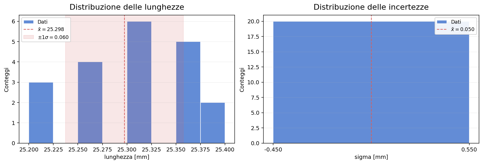
Comparison across two axes
When you pass ax, mespy draws on the existing subplot and lets you combine multiple distributions in the same figure without changing the API.
fig, (ax_left, ax_right) = plt.subplots(
    1,
    2,
    figsize=(12, 4),
    dpi=140,
    constrained_layout=True,
)

mp.histogram(
    lunghezza,
    bins=8,
    xlabel="lunghezza [mm]",
    title="Distribuzione delle lunghezze",
    ax=ax_left,
)

mp.histogram(
    sigma,
    bins="sqrt",
    xlabel="sigma [mm]",
    title="Distribuzione delle incertezze",
    show_band=False,
    ax=ax_right,
)

fig